The circumference of an ellipse

This notebook is inspired by Matt Parker's video on the same topic. Notebook by Luka van der Plas.

You are (hopefully) familiar with the formula to calculate the circumference of a circle. If we have a circle with radius $r$...

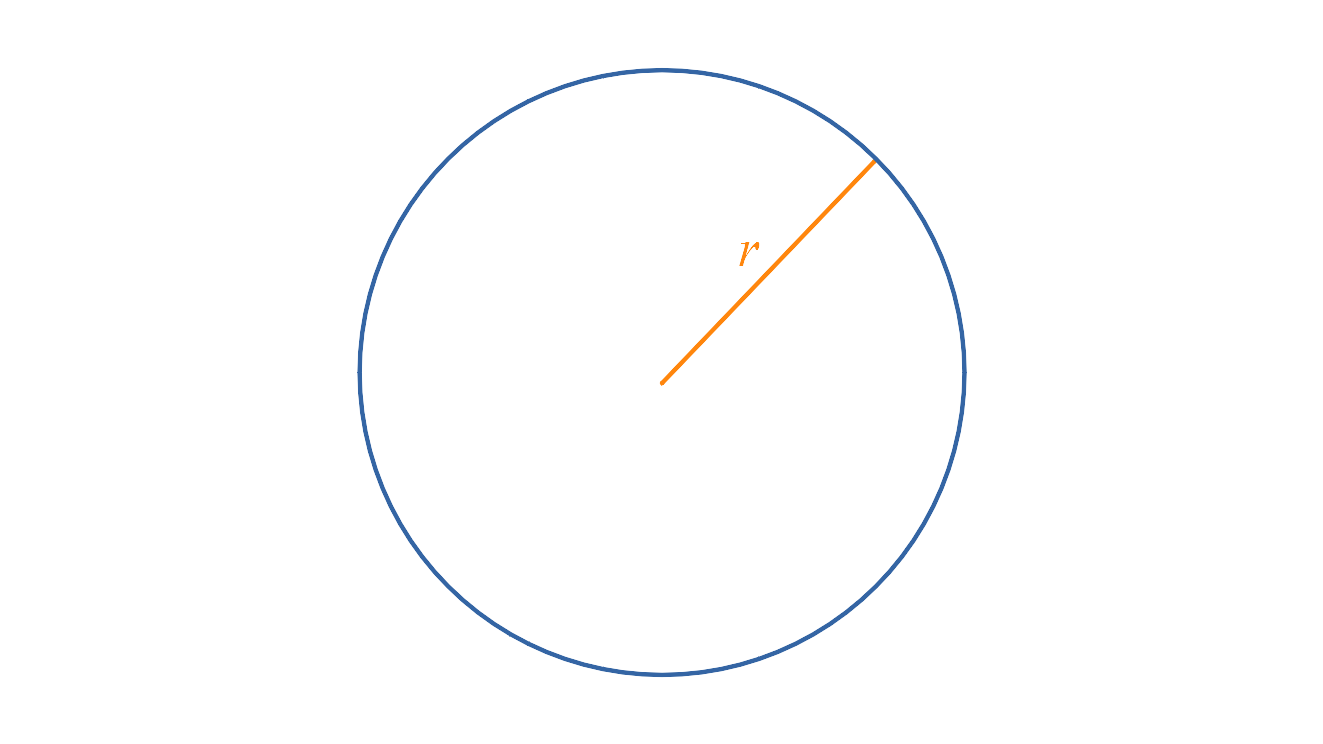
... then the circumference $C$ is equal to $2\pi r$.

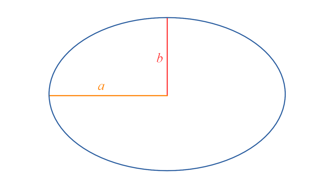
But what is the formula for an ellipse?

Because an ellipse is elongated, we can't just describe it with a single value for the radius. Instead, we give the semi-major axis, $a$, and the semi-minor axis, $b$.

(The semi-bit means that we go form the centre to the edge, not from one edge to the other. So $a$ and $b$ are analogous to the radius, not the diameter.)

Let's start by making a structure for that.

Our Ellipse struct stores the valus of $a$ and $b$. I also defined some constructors. If you give the values of $a$ and $b$, the constructor will check if $a$ is not smaller than $b$, and give you an error otherwise.

You can also make an ellipse by just given a value for $a$. We then assume that $b=1$.

Okay, let's make an ellipse!

You can retrieve the values of the axes by putting .a or .b behind the name.

These values are really all we need to do some geometry. But it's probably nice to have some visualisation as well. Here is a picture of our ellipse:

Beautiful.

Now, let's go back to our question: how do we calculate the circumference of an ellipse?

Surprisingly, there is no neat formula! There are some infinite series, but those are not exactly easy to use. For example, we can calculate the circumference $C$ using the following formula:

$$C=\pi (a+b)(1+\sum _{n=1}^{\mathrm{\infty }}(\frac{(2n-1)!!}{2^{n}n!}{)}^2\frac{h^n}{(2n-1{)}^2})$$

where

$$h=\frac{(a-b{)}^2}{(a+b{)}^2}$$

Oof.

Don't worry about understanding the formula. One thing of note: the formula contains an infinite sum (note the $\infty$ sign above the $\mathrm{\Sigma }$). We can't actually repeat a calculation into infinity, but the more steps we make, the closer the result will be to the actual circumference. In fact, for any level of precision that we want, we can find a number of steps that will guarantee that precision.

This formula is a hassle to encode in a Julia in the 21st century. (Don't worry, I already did that for you.) But using a formula like that was even worse in History Times, when people did not have computers at their disposal. So instead, people would use approximation functions.

An approximation function will give you something close to the real circumference, but it's easier to calculate. That is what we will do in this notebook! We can encode some functions and compare them to the "true" value of the circumference.

Approximations

Let's define some approximation functions. A function should take an ellipse as input, and return the circumference. Here is a simple example:

To compare these functions, we will keep them in a Dict. This one will store a good name for the function, and the function itself. The names will be useful when we make a plot.

Some more functions. You can add more your own (see Matt's video for inspiration), or even try to find the best function you can!

(Remember that if you want to add a function to the plot below, you have to include it in the approximations dict.)

Results

This plot shows how all of our functions are doing.

We are interested in the error of our function, i.e. how far it is from the real circumference. In this plot, we compare it to the ratio $\frac{a}{b}$, so we can see how well it does in ellipses with various shapes. If the ratio is 1, we just have a circle. The higher the ratio, the more elongated our ellipse is.

Here are some options for your plot:

Maximum error:

What should be the limit on the y axis?

Maximum $\frac{a}{b}$ ratio:

What should be the limit on the x-axis?

Number of data points:

Slide up if you want more precision in the plot, slide down if you want to speed up calculations.

The true circumference

If you are interested, here is the code I used to calculate the "true" circumference and to compare that with the approximations.

Though you probably remember the formula, this is the infinite series we can use to get the true circumference.

$$C=\pi (a+b)(1+\sum _{n=1}^{\mathrm{\infty }}(\frac{(2n-1)!!}{2^{n}n!}{)}^2\frac{h^n}{(2n-1{)}^2})$$

where

$$h=\frac{(a-b{)}^2}{(a+b{)}^2}$$

As I mentioned, you can sum to a particular value of $n$ to get the level of precision that you want. I used $n=10$.

To create the plot, we generate a range of values for the $\frac{a}{b}$ ratio and calculate the "true" circumference for each.

For a particular approximation function, we can get the errors by applying the function to each ratio, and substracting the true circumference from the result.

To get the relative error, we also divide by the circumference.

Lastly, here is the function I used to display the ellipse in the beginning.